Categories
Distillation control Dynamic Modeling Kotlin Model-View-Controller TornadoFX User Interface

Column Simulation Revisited

Background

Earlier this year I posted the description, and implementation, of a distillation column simulation. The focus then was on object-oriented modeling in dynamic simulations. I collected the results of a 16 hour run in arrays which were later plotted using Let’s plot.

Since then I have come to appreciate TornadoFX as a UI tool. In my most recent post I showed how it is possible to build an interactive simulation app to plot the results of a fairly simple model, namely Burgers’ Equation. The simulation was batch in the sense that it only ran for a pre-specified amount of time. Thus, while interactive, this feature had somewhat limited use (e.g. “Pause”, “Resume”, and “Speed up” for example). The real benefit of interactive is for continuous time simulations. As I will show here, this can be done with TornadoFX as well.

The ideal candidate for continuous time simulation is a model of a continuously operating process. The distillation column is such a candidate. Now let me make another plug for MVC. Because I always separate the model from the UI, I could readily take the exact same distillation column model, that I had previously used with Let’s plot, and now use it with TornadoFX.

Results

Since I had the model and the basic forms of the View and ViewController, I could build on those pieces to enhance the interface as shown below:
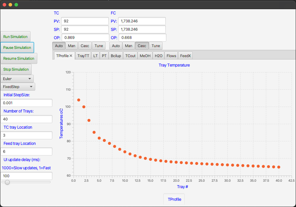
Interactive user interface for distillation column simulation.

As you can see I have kept most of the controls on the left panel but added several more plot-tabs in addition to two (PID)-controller faceplates. I attach a short video of how I use the interface.

Video showing the use of the column simulation interface.

Implementation

In the spirit of sharing and teaching I show most of the relevant code for making this interface. For example, the code below is the entire code for the main view. Notice that it describes only what you will see, not how the UI responds. The latter is the task for the ViewController.

The layout in this case is guided by three very useful items: “border pane”, “vbox”, and “hbox”. The border pane gives the overall structure of the interface, whereas the two boxes are used to position related items either vertically or horizontally. By alternating the use of these boxes you can get your buttons and fields to fall in whichever place you desire.

Both buttons and textfields have the option to use an “action” in which you call the appropriate function in the ViewController to respond to user requests.

package view

import controller.ViewController
import javafx.geometry.Pos
import javafx.scene.chart.NumberAxis
import javafx.scene.layout.Priority
import tornadofx.*

var viewController = find(ViewController::class)

class MainView: View() {
    override val root = borderpane {
        left = vbox {
            alignment = Pos.CENTER_LEFT
            button("Run Simulation") {
                action {
                    viewController.runSimulation()
                }
            }
            button("Pause Simulation") {
                action {
                    viewController.pauseSimulation()
                }
            }
            button("Resume Simulation") {
                action {
                    viewController.resumeSimulation()
                }
            }
            button("Stop Simulation") {
                action {
                    viewController.endSimulation()
                }
            }
            combobox(viewController.selectedDiscretizer, viewController.dicretizers)
            combobox(viewController.selectedStepController, viewController.stepControllers)
            label("  Initial StepSize:")
            textfield(viewController.initStepSize)
            label("  Number of Trays:")
            textfield(viewController.numberOfTrays)
            label("  TC tray Location")
            textfield(viewController.temperatureTrayLocation)
            label("  Feed tray Location")
            textfield(viewController.feedTrayLocation)
            label("  UI update delay (ms):")
            label("1000=Slow updates, 1=Fast")
            textfield(viewController.simulator.sliderValue)
            slider(min=1, max=1000, value = viewController.simulator.sliderValue.value) {
                bind(viewController.simulator.sliderValue)
            }
        }
        center = vbox {
            hbox {
                vbox {
                    label("TC")
                    hbox {
                        label("PV:")
                        textfield(viewController.tc.pv)
                    }
                    hbox {
                        label("SP:")
                        textfield(viewController.tc.sp) {
                            action {
                                viewController.tc.newSP()
                            }
                        }
                    }
                    hbox {
                        label("OP:")
                        textfield(viewController.tc.op) {
                            action {
                                viewController.tc.newOP()
                            }
                        }
                    }
                    hbox {
                        togglebutton("Auto", viewController.tc.toggleGroup) {
                            action { viewController.tc.modeChange() }
                        }
                        togglebutton("Man", viewController.tc.toggleGroup) {
                            action { viewController.tc.modeChange() }
                        }
                        togglebutton("Casc", viewController.tc.toggleGroup) {
                            action { viewController.tc.modeChange() }
                        }
                        togglebutton("Tune", viewController.tc.toggleGroup) {
                            action { viewController.tc.modeChange() }
                        }
                    }
                }
                vbox {
                    label("FC")
                    hbox {
                        label("PV:")
                        textfield(viewController.fc.pv)
                    }
                    hbox {
                        label("SP:")
                        textfield(viewController.fc.sp) {
                            action {
                                viewController.fc.newSP()
                            }
                        }
                    }
                    hbox {
                        label("OP:")
                        textfield(viewController.fc.op) {
                            action {
                                viewController.fc.newOP()
                            }
                        }
                    }
                    hbox {
                        togglebutton("Auto", viewController.fc.toggleGroup) {
                            action { viewController.fc.modeChange() }
                        }
                        togglebutton("Man", viewController.fc.toggleGroup) {
                            action { viewController.fc.modeChange() }
                        }
                        togglebutton("Casc", viewController.fc.toggleGroup) {
                            action { viewController.fc.modeChange() }
                        }
                        togglebutton("Tune", viewController.fc.toggleGroup) {
                            action { viewController.fc.modeChange() }
                        }
                    }
                }
            }
            tabpane {
                vgrow = Priority.ALWAYS
                tab("TProfile") {
                    scatterchart("Tray Temperature", NumberAxis(), NumberAxis()) {
                        //createSymbols = false
                        yAxis.isAutoRanging = false
                        val xa = xAxis as NumberAxis
                        xa.lowerBound = 1.0
                        xa.upperBound = 40.0
                        xa.tickUnit = 5.0
                        xa.label = "Tray #"
                        val ya = yAxis as NumberAxis
                        ya.lowerBound = 60.0
                        ya.upperBound = 120.0
                        ya.tickUnit = 10.0
                        ya.label = "Temperatures oC"
                        series("TProfile") {
                            data = viewController.tempProfile
                        }
                    }
                }
                tab("TrayTT") {
                    linechart("Tray Temperature", viewController.xAxisArray[0], NumberAxis()) {
                        createSymbols = false
                        yAxis.isAutoRanging = false
                        val ya = yAxis as NumberAxis
                        ya.lowerBound = 65.0
                        ya.upperBound = 120.0
                        ya.tickUnit = 5.0
                        ya.label = "Temperatures oC"
                        series("Temperature") {
                            data = viewController.tempList
                        }
                    }
                }
                tab("LT") {
                    linechart("Levels", viewController.xAxisArray[1], NumberAxis()) {
                        createSymbols = false
                        yAxis.isAutoRanging = false
                        val ya = yAxis as NumberAxis
                        ya.lowerBound = 40.0
                        ya.upperBound = 80.0
                        ya.tickUnit = 10.0
                        ya.label = "Level %"
                        series("Reboiler Level") {
                            data = viewController.reboilLevelList
                        }
                        series("Condenser Level") {
                            data = viewController.condenserLevelList
                        }
                    }
                }
                tab("PT") {
                    linechart("Column Pressure", viewController.xAxisArray[2], NumberAxis()) {
                        createSymbols = false
                        yAxis.isAutoRanging = false
                        val ya = yAxis as NumberAxis
                        ya.lowerBound = 0.75
                        ya.upperBound = 1.25
                        ya.tickUnit = 0.05
                        ya.label = "Pressure, atm"
                        series("Pressure") {
                            data = viewController.pressureList
                        }
                    }
                }
                tab("Boilup") {
                    linechart("Reboiler Boilup", viewController.xAxisArray[3], NumberAxis()) {
                        createSymbols = false
                        yAxis.isAutoRanging = false
                        val ya = yAxis as NumberAxis
                        ya.lowerBound = 1500.0
                        ya.upperBound = 2000.0
                        ya.tickUnit = 100.0
                        ya.label = "Flow, kmol/h"
                        series("Temperature") {
                            data = viewController.boilupList
                        }
                    }
                }
                tab("TCout") {
                    linechart("TC output signal", viewController.xAxisArray[4], NumberAxis()) {
                        createSymbols = false
                        yAxis.isAutoRanging = false
                        val ya = yAxis as NumberAxis
                        ya.lowerBound = 60.0
                        ya.upperBound = 100.0
                        ya.tickUnit = 10.0
                        ya.label = "Signal value %"
                        series("TCout") {
                            data = viewController.tcOutList
                        }
                    }
                }
                tab("MeOH") {
                    linechart("Methanol in Reboiler", viewController.xAxisArray[5], NumberAxis()) {
                        createSymbols = false
                        yAxis.isAutoRanging = false
                        val ya = yAxis as NumberAxis
                        ya.lowerBound = 0.0
                        ya.upperBound = 10000.0
                        ya.tickUnit = 2000.0
                        ya.label = "ppm"
                        series("MeOH") {
                            data = viewController.meohBtmsList
                        }
                    }
                }
                tab("H2O") {
                    linechart("Water in condenser", viewController.xAxisArray[6], NumberAxis()) {
                        createSymbols = false
                        yAxis.isAutoRanging = false
                        val ya = yAxis as NumberAxis
                        ya.lowerBound = 0.0
                        ya.upperBound = 400.0
                        ya.tickUnit = 50.0
                        ya.label = "ppm"
                        series("H2O") {
                            data = viewController.h20OHList
                        }
                    }
                }
                tab("Flows") {
                    linechart("Feed, Btms and Dist flow", viewController.xAxisArray[7], NumberAxis()) {
                        createSymbols = false
                        yAxis.isAutoRanging = false
                        val ya = yAxis as NumberAxis
                        ya.lowerBound = 0.0
                        ya.upperBound = 2000.0
                        ya.tickUnit = 200.0
                        ya.label = "kmol/h"
                        series("Feed") {
                            data = viewController.feedRateList
                        }
                        series("Btms") {
                            data = viewController.btmsFlowList
                        }
                        series("Dist") {
                            data = viewController.distList
                        }

                    }
                }
                tab("FeedX") {
                    linechart("MeOH in Feed", viewController.xAxisArray[8], NumberAxis()) {
                        createSymbols = false
                        yAxis.isAutoRanging = false
                        val ya = yAxis as NumberAxis
                        ya.lowerBound = 30.0
                        ya.upperBound = 60.0
                        ya.tickUnit = 5.0
                        ya.label = "Composition, mole-%"
                        series("FeedX") {
                            data = viewController.feedCmpList
                        }
                    }
                }

            }
        }
    }
}

I’m not showing the ViewController code here as it is quite similar to what I had previously shown in my most recent post. However, there is a piece of new code that is quite important and sits between the model and the interface. This is a class to handle the display and actions of the PID-controller faceplates. This code is shown here.

package controller

import instruments.ControlMode
import instruments.PIDController
import javafx.beans.property.SimpleDoubleProperty
import javafx.scene.control.ToggleButton
import javafx.scene.control.ToggleGroup

class PIDViewController(var pid: PIDController) {
    val pv = SimpleDoubleProperty(pid.pv)
    val sp = SimpleDoubleProperty(pid.sp)
    val op = SimpleDoubleProperty(pid.output)
    var mode = "Auto"

    val toggleGroup = ToggleGroup()
    fun update() {
        pv.value = pid.pv
        if (mode != "Man") {
            op.value = pid.output
        }
        if (mode == "Casc" || mode == "Man") {
            sp.value = pid.sp
        }
    }
    fun modeChange() {
        val button = toggleGroup.selectedToggle as? ToggleButton
        val buttonText = button?.text ?: "Null"
        when (buttonText) {
            "Auto" -> {
                pid.controllerMode = ControlMode.automatic
                mode = "Auto"
            }
            "Man" -> {
                pid.controllerMode = ControlMode.manual
                mode = "Man"
            }
            "Casc" -> {
                pid.controllerMode = ControlMode.cascade
                mode = "Casc"
            }
            "Tune" -> {
                pid.controllerMode = ControlMode.autoTune
                mode = "Tune"
            }
            else -> {}
        }
    }
    fun newSP() {
        pid.sp = sp.value
    }
    fun newOP() {
        pid.output = op.value
    }
}

This class is akin to a view controller in that has properties that can be displayed in the main interface. However, it also owns a reference to an actual PID controller in the process model. That way we can interactively interpret user input and convey them to the model.

Conclusions

Interactive dynamic simulations are extremely useful tools in the exploration, understanding and control of real processes. Over the years I have built many models with different interfaces for different platforms. I find Kotlin and TornadoFX to be a very powerful combination for desktop applications compiled for the JVM.
Categories
Dynamic Modeling Kotlin Model-View-Controller TornadoFX User Interface

Building an Interactive Process Simulator from Scratch

Introduction

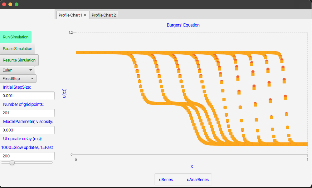
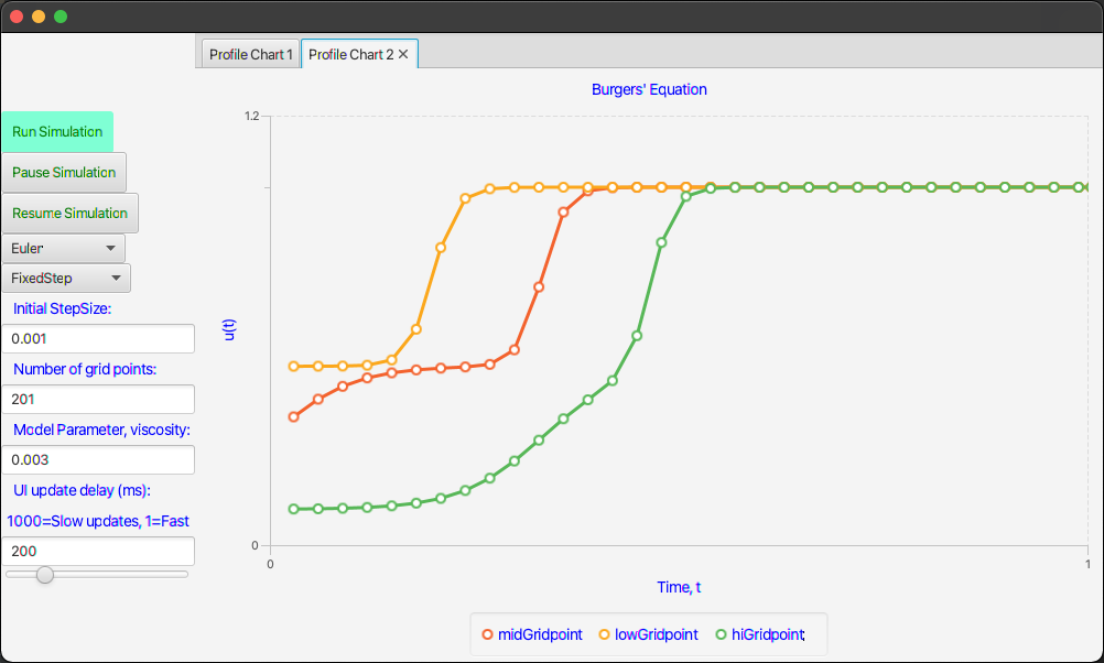
In previous posts I have introduced dynamic integration techniques, MVC designs, Kotlin and TornadoFX. It is now time to put all the pieces together in a free-standing app with a responsive user interface. The final result will look like these two screen shots.

Figure 1. User interface with time dependent velocity profiles shown.
Figure 2. Tab 2 of the UI showing the fluid velocity as a function of time at three different x-positions.

Let’s get started putting this app together piece by piece.

Create the Project Template

In previous posts I have shown how to do this so I will move quickly through this section.

Step 1. Make a new project with JetBrains IntelliJ.

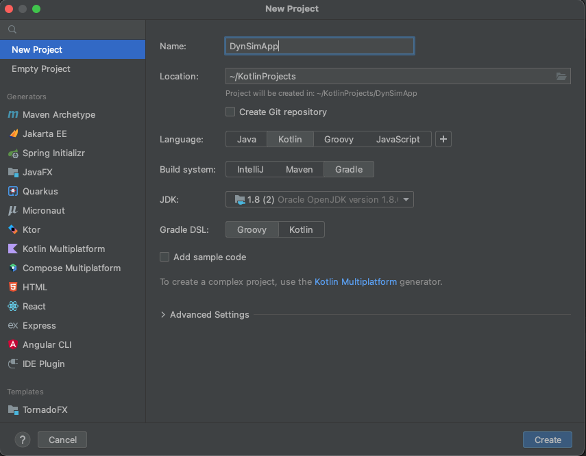
Figure 3. The new project screen. Use Kotlin, Gradle, Groovy and JDK 1.8

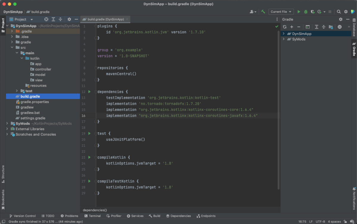
Step 2. Link the project to any local, supporting projects you might have (in my case SyMods), assign dependencies in build.gradle and finally provide empty folders (packages) for the “app”, “model”, “view” and the “controller” as in MVC.

Figure 4. Model structure ready for source files.

Since the build.gradle is such an important part of the project I show the script more clearly here:

plugins {
    id 'org.jetbrains.kotlin.jvm' version '1.7.10'
}

group = 'org.example'
version = '1.0-SNAPSHOT'

repositories {
    mavenCentral()
}

dependencies {
    testImplementation 'org.jetbrains.kotlin:kotlin-test'
    implementation 'org.example:SyMods'
    implementation 'no.tornado:tornadofx:1.7.20'
    implementation "org.jetbrains.kotlinx:kotlinx-coroutines-core:1.6.4"
    implementation "org.jetbrains.kotlinx:kotlinx-coroutines-javafx:1.6.4"
}

test {
    useJUnitPlatform()
}

compileKotlin {
    kotlinOptions.jvmTarget = '1.8'
}

compileTestKotlin {
    kotlinOptions.jvmTarget = '1.8'
}

The Model

In most versions of MVC designs, the model is the only part that is completely independent of the other pieces. In other words, the model has no knowledge of either the view or the (view-) controller. The only contract the model has with the outside world is that it implements the Integratable interface. That way the same model, without substantial modifications, can be used with a completely different user interface implementation (e.g. Java/Swing or Swift/Cocoa).

The model I have chosen for this example is borrowed from the field of fluid dynamics. Such systems are described by a set of nonlinear partial differential equations expressing the conservation of mass and momentum for incompressible Newtonian fluids. The fluid velocity in three dimensions is captured in the Navier Stokes equation of fluid dynamics (see Ref. 1 for a complete derivation).

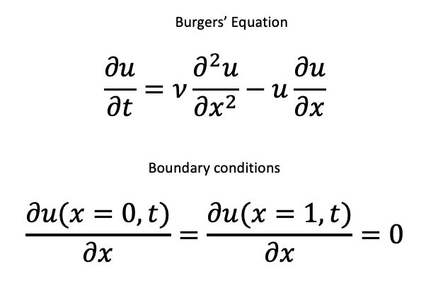
If we limit the flow model to the fluid velocity component in one dimension, and neglect pressure and gravitational effects, we obtain the one-dimensional Burgers’ equation.

Figure 5. Model of the one-dimensional velocity component, u, for a viscous fluid.

We can think of this equation as representing the velocity in the x-direction as the fluid is moving freely along a path. Note that the fluid is viscous as captured by the kinematic viscosity, v (m^2/s).

According to Ref. 1, Burgers’ equation is a standard test problem for numerical methods for two reasons (1) It is a nonlinear equation with known analytical solutions, (2) It can be made increasingly more difficult to solve numerically as the viscosity decreases.

The equation is first order in time and second order in space. Thus, it requires one initial condition and two boundary conditions. The initial condition is taken from the analytical solution at time = 0. The boundary conditions are shown above. They state that the spatial velocity derivative is zero at both ends of the flow path at all times.

Numerical techniques for solving partial differential equations like this typically involve breaking up the x-direction in a large number (N-1) of small segments, dx, flanked by N grid points to help with the approximation of the spatial derivatives. This way we end up with a set of N ordinary differential equations that can be solved with standard integrators such as Euler or Runge-Kutta.

For this example I’m choosing to use a Spline Collocation Method to approximate the first and second order spatial derivatives (See Ref. 2 for details of this method). The complete code for the model is shown here:

package model

import integrators.Integratable
import utilities.derivativesAtGridpoints
import kotlin.math.exp

class BurgersEquation(var nGridPoints: Int): Integratable {

    val length = 1.0
    var dx = length / (nGridPoints - 1)
    var time = 0.0
    var vis = 0.003
    var x = DoubleArray(nGridPoints) { it * dx }
    var u = DoubleArray(nGridPoints) { phi(x[it], time) }

    override fun initialConditionsUsingArray(xin: DoubleArray): DoubleArray {
        x = DoubleArray(nGridPoints) { it * dx }
        val u0 = xin.copyOf()
        for (i in 0 until nGridPoints) {
            u0[i] = phi(this.x[i], time)
        }
        return u0
    }

    override fun updateStatesFromStateVector(x: DoubleArray, time: Double) {
        this.time = time
        u = x
    }

    override fun updateDerivativeVector(df: DoubleArray, time: Double): DoubleArray {
        val ux = derivativesAtGridpoints(xL=0.0, xU=length, n=nGridPoints, u=u).b
        ux[0] = 0.0
        ux[nGridPoints-1] = 0.0
        val uxx = derivativesAtGridpoints(xL=0.0, xU=length, n=nGridPoints, u=ux).b
        val ut = df.copyOf()
        for (i in 0 until nGridPoints) {
            ut[i] = vis * uxx[i] - u[i] * ux[i]
        }
        return ut
    }

    override fun dimension(): Int {
        return nGridPoints
    }

    override fun stiff(): Boolean {
        return false
    }

    fun phi(x: Double, t: Double): Double {
        //
        // Function phi computes the exact solution of Burgers' equation
        // for comparison with the numerical solution.  It is also used to
        // define the initial and boundary conditions for the numerical
        // solution.
        //
        // Analytical solution
        val a = (0.05 / vis) * (x - 0.5 + 4.95 * t)
        val b = (0.25 / vis) * (x - 0.5 + 0.75 * t)
        val c = (0.5 / vis) * (x - 0.375)
        val ea = exp(-a)
        val eb = exp(-b)
        val ec = exp(-c)
        return (0.1 * ea + 0.5 * eb + ec) / (ea + eb + ec)
    }
}

The View

Next to the model, the view is similarly isolated from the other software components. In particular, it has no direct knowledge of the model implementation. This is important from a code reuse point of view. For example, it would be quite easy to use this view for another model by just changing a few text labels.

I’m using TornadoFX to build the interface. Without further explanations of the code, I think you can see how the declarative statements below result in the interfaces shown in Figures 1 and 2.

package view

import controller.ViewController
import javafx.geometry.Pos
import javafx.scene.chart.NumberAxis
import tornadofx.*

var viewController = find(ViewController::class)

class MainView: View() {
    override val root = borderpane {
        left = vbox {
            alignment = Pos.CENTER_LEFT
            button("Run Simulation") {
                action {
                    viewController.runSimulation()
                }
            }
            button("Pause Simulation") {
                action {
                    viewController.pauseSimulation()
                }
            }
            button("Resume Simulation") {
                action {
                    viewController.resumeSimulation()
                }
            }
            combobox(viewController.selectedDiscretizer, viewController.dicretizers)
            combobox(viewController.selectedStepController, viewController.stepControllers)
            label("  Initial StepSize:")
            textfield(viewController.initStepSize)
            label("  Number of grid points:")
            textfield(viewController.nGridPoints)
            label("  Model Parameter, viscosity:")
            textfield(viewController.viscosity)
            label("  UI update delay (ms):")
            label("1000=Slow updates, 1=Fast")
            textfield(viewController.simulator.sliderValue)
            slider(min=1, max=1000, value = viewController.simulator.sliderValue.value) {
                bind(viewController.simulator.sliderValue)
            }
        }
        center = tabpane {
            tab("Profile Chart 1") {
                scatterchart("Burgers' Equation", NumberAxis(), NumberAxis()) {
                    xAxis.isAutoRanging = false
                    val xa = xAxis as NumberAxis
                    xa.lowerBound = 0.0
                    xa.upperBound = 1.0
                    xa.label = "x"
                    yAxis.isAutoRanging = false
                    val ya = yAxis as NumberAxis
                    ya.lowerBound = 0.0
                    ya.upperBound = 1.2
                    ya.label = "u(x,t)"
                    series("uSeries") {
                        data = viewController.uSeriesData
                    }
                    series("uAnalSeries") {
                        data = viewController.uAnalSeriesData
                    }
                }
            }
            tab("Profile Chart 2") {
                linechart("Burgers' Equation", NumberAxis(), NumberAxis()) {
                    xAxis.isAutoRanging = false
                    val xa = xAxis as NumberAxis
                    xa.lowerBound = 0.0
                    xa.upperBound = 1.0
                    xa.label = "Time, t"
                    yAxis.isAutoRanging = false
                    val ya = yAxis as NumberAxis
                    ya.lowerBound = 0.0
                    ya.upperBound = 1.2
                    ya.label = "u(t)"
                    series("midGridpoint") {
                        data = viewController.midGridpointData
                    }
                    series("lowGridpoint") {
                        data = viewController.lowGridpointData
                    }
                    series("hiGridpoint") {
                        data = viewController.hiGridpointData
                    }
                }
            }
        }
    }
}

A couple of important comments on the view code:

  • There is no explicit mention of any of the UI classes like Button, Label, TextField etc.. Instead, these are created implicitly from TornadoFX’s builder functions.
  • There is no procedural code in the view, only configuration statements.
  • Values in and out of the interface go through the viewController. The controller is injected into the view by the statement var viewController = find(ViewController::class)
  • The view component values and the viewController variables are connected through bindings. Bindings allow for automatic transfer of updated information without having to write code to detect changes and transfer new values from one object to another.

Anyone who has worked with Java/Swing or Java/JavaFX will appreciate how simple it is to build an interface with Kotlin/TornadoFX.

View – Styling

While it is possible to provide styling code directly into the view functions I find that view code becomes less clear. An alternative that I like is to list the styling attributes in a separate Stylesheet class. This is what I used for the example application:

package app

import javafx.scene.paint.Color
import javafx.scene.text.FontWeight
import tornadofx.*

class Styles : Stylesheet() {
    init {
        button {
            padding = box(10.px)
            textFill = c("green")
            and(hover) {
                backgroundColor += Color.AQUAMARINE
            }
        }

        label {
            padding = box(5.px)
            fontSize = 14.px
            fontWeight = FontWeight.BOLD
            textFill = c("blue")
        }
    }
}

I have only done the most basic of what you can achieve with these Stylesheets. For example, I specify how much padding the buttons should have and their text color. I also specify the desired color change when the mouse “hovers” over them. Similar decorations for the labels are also shown.

The Controller

The controller usually takes a very central position in most MVC designs. In my version it owns the model and it is injected into the view as I mentioned above. The controller is also an Observer of the Simulator (see below). As such it implements the IObserver‘s update(…) function. This function is called from the Simulator when changes in the model’s data have taken place and need to be displayed. Recall that the model does not know about the view and therefore has no direct way of communicating with it. All communication between the model and the view must pass through the controller.

The controller implements a few JavaFX and TornadoFX data structures that are observable to view items through bindings. For example, take the uSeriesData in the controller. It holds data for one of the series in the view’s Profile Chart 1. This is how we use it in the view:

series("uSeries") {
      data = viewController.uSeriesData
}

In the controller this variable is a special ArrayList and is declared as follows:

var uSeriesData = FXCollections.observableArrayList<XYChart.Data<Number, Number>>()

When the Simulator sends the controller an update(…) request, the uSeriesData array is updated based on information it finds in the model.

if (updateCounter > updateFrequency || updateCounter == 0) {
      for (i in 0 until model.nGridPoints) {
           val xValue = model.x[i]
           uSeriesData.add(XYChart.Data(xValue, model.u[i]))
       }
       updateCounter = 1
 }

The neat feature about these data structures is that they are “observable” in the sense that the chart updates automatically as soon as the controller makes new data available in the uSeriesData array. Similarly, when data items are removed from the array, the display changes accordingly. In other words, there is no need to explicitly “refresh” the charts with user code. Ref 3. is a good source to learn about these data structures and their use in JavaFX/TornadoFX applications.

package controller

import utilities.IObserver
import javafx.beans.property.SimpleDoubleProperty
import javafx.beans.property.SimpleIntegerProperty
import javafx.beans.property.SimpleStringProperty
import javafx.collections.FXCollections
import javafx.scene.chart.XYChart
import model.BurgersEquation
import model.Simulator
import tornadofx.*


class ViewController: Controller(), IObserver {

    var model = BurgersEquation(201)
    var endTime = 1.0
    var simulator = Simulator(model)

    var uSeriesData = FXCollections.observableArrayList<XYChart.Data<Number, Number>>()
    var uAnalSeriesData = FXCollections.observableArrayList<XYChart.Data<Number, Number>>()
    var midGridpointData = FXCollections.observableArrayList<XYChart.Data<Number, Number>>()
    var lowGridpointData = FXCollections.observableArrayList<XYChart.Data<Number, Number>>()
    var hiGridpointData = FXCollections.observableArrayList<XYChart.Data<Number, Number>>()


    val dicretizers = FXCollections.observableArrayList("Euler", "RungeKutta", "RKFehlberg")
    val stepControllers = FXCollections.observableArrayList("FixedStep", "VariableStep")
    val selectedDiscretizer = SimpleStringProperty("Euler")
    val selectedStepController = SimpleStringProperty("FixedStep")
    val initStepSize = SimpleDoubleProperty(0.001)
    val nGridPoints = SimpleIntegerProperty(model.nGridPoints)
    val viscosity = SimpleDoubleProperty(model.vis)

    var updateCounter = 0
    val updateFrequency = 4

    init {
        simulator.addIObserver(this)
    }

    fun runSimulation() {
        model = BurgersEquation(nGridPoints.value)
        model.vis = viscosity.value
        simulator.ode = model
        simulator.discretizer = selectedDiscretizer.value
        simulator.stepSizeType = selectedStepController.value
        simulator.initialStepSize = initStepSize.value
        simulator.runSimulation()
    }

    fun pauseSimulation() {
        simulator.pauseSimulation()
    }

    fun resumeSimulation() {
        simulator.resumeSimulation()
    }

    override fun update(theObserved: Any?, changeCode: Any?) {
        val code = changeCode as String
        when (code) {
            "reset" -> {
                if (uSeriesData.size > 1) {
                    uSeriesData.remove(0, uSeriesData.size)
                    uAnalSeriesData.remove(0, uAnalSeriesData.size)
                    midGridpointData.remove(0, midGridpointData.size)
                    lowGridpointData.remove(0, lowGridpointData.size)
                    hiGridpointData.remove(0, hiGridpointData.size)
                }
            }
            else -> {
                val time = model.time
                if (updateCounter > updateFrequency || updateCounter == 0) {
                    for (i in 0 until model.nGridPoints) {
                        val xValue = model.x[i]
                        uSeriesData.add(XYChart.Data(xValue, model.u[i]))
                        uAnalSeriesData.add(XYChart.Data(xValue, model.phi(x = xValue, t = time)))
                    }
                    updateCounter = 1
                }
                updateCounter += 1
                val midGridpoint = model.nGridPoints / 2
                val lowGridpoint = midGridpoint - 20 * model.nGridPoints / 201
                val hiGridpoint = midGridpoint + 20 * model.nGridPoints / 201
                midGridpointData.add(XYChart.Data(time, model.u[midGridpoint]))
                lowGridpointData.add(XYChart.Data(time, model.u[lowGridpoint]))
                hiGridpointData.add(XYChart.Data(time, model.u[hiGridpoint]))
            }
        }
    }
}

There are a few more modules we have to discuss before the app is complete. One of these is the Simulator.

The Simulator

This module is most closely characterized as a model but it is generic enough that it can be treated separately. The simulator is responsible for the numerical integration and for notifying the controller when is time to sample the model for new data to display.

The simulator is generic in the sense that it can integrate any model as long as the model implements the Integratable interface. The simulator itself implements the interface IObservable which means that it can keep track of, and notify, observing objects (e.g. the controller).

An important task for the simulator is to start the integration and run it to completion without blocking the user from working with the UI. Traditionally this is done by starting a low priority background Thread. However, threads can be tricky to work with, especially around shared data. Instead I have opted to use Kotlin’s Coroutine package. Ref. 4 is the perfect source to learn about coroutines. Here I will only highlight the features I have used.

Coroutines are launched in a CoroutineScope. For UI applications it is quite useful to derive a private scope from the general CoroutineScope() but specify that we want the coroutine to be dispatched on the JavaFx UI thread.

import kotlinx.coroutines.*
import kotlinx.coroutines.javafx.JavaFx


class Simulator(var ode: Integratable) : IObservable {

    private var job = Job()
    private val myScope: CoroutineScope =     CoroutineScope(Dispatchers.JavaFx + job)
                :
                :
                :
}

We use the private scope to launch a coroutine with code provided in the trailing lambda.

        myScope.launch {
            while (time <= endTime) {
                time = integrator.currentTime
                integrator.startTime = time
                integrator.endTime = time + dt
                integrator.continueCalculations()
                            :
                            :
                            :
            }
        }

You can easily identify these code snippets in their complete context of the Simulator code below. The coroutines are quite nice for dynamic simulations like this because we can implement start, stop, pause, resume, etc. without freezing the UI or making it sluggish.

package model

import integrators.DiscretizationModel
import integrators.Integratable
import integrators.IntegrationServer
import integrators.StepSizeControlModel
import javafx.beans.property.SimpleDoubleProperty
import utilities.IObservable
import utilities.IObserver
import utilities.ObservableComponent
import kotlinx.coroutines.*
import kotlinx.coroutines.javafx.JavaFx


class Simulator(var ode: Integratable) : IObservable {
    private val myObservableComponent: ObservableComponent = ObservableComponent()
    private var job = Job()
    private val myScope: CoroutineScope = CoroutineScope(Dispatchers.JavaFx + job)

    val sliderValue = SimpleDoubleProperty(200.0)
    var sliderValueInt: Long = 200

    lateinit var integrator: IntegrationServer
    var discretizer = "Euler"
    var stepSizeType = "FixedStep"
    lateinit var discretizationType: DiscretizationModel
    lateinit var stepSizeControlType: StepSizeControlModel
    var time = 0.0
    var endTime = 1.0
    var reportingInterval = 0.1
    var dt = reportingInterval / 10
    var dt0 = dt
    var initialStepSize = 0.001
    var simulationPaused = false
    var endSimulation = false
    private var reportTimer = 0.0
    var x: DoubleArray

    init {
        val dim = ode.dimension()
        x = DoubleArray(dim)
        System.arraycopy(ode.initialConditionsUsingArray(x), 0, x, 0, dim)
    }

    fun reset() {
        discretizationType = when(discretizer) {
            "RungeKutta" -> DiscretizationModel.ClassicalRK
            "RKFehlberg" -> DiscretizationModel.RKFehlberg
            else -> DiscretizationModel.ModifiedEuler
        }
        stepSizeControlType = when(stepSizeType) {
            "VariableStep" -> StepSizeControlModel.VariableStepController
            else -> StepSizeControlModel.FixedStepController
        }
        x = DoubleArray(ode.dimension())
        System.arraycopy(ode.initialConditionsUsingArray(x), 0, x, 0, ode.dimension())
        integrator = IntegrationServer(discretizationType, stepSizeControlType);
        integrator.ode = ode

        integrator.initialStepSize = initialStepSize
        integrator.accuracy = 1.0e-5
        reportingInterval = 0.03
        dt = reportingInterval / 2
        dt0 = dt

        time = 0.0
        reportTimer = 0.0
        integrator.startTime = 0.0
        integrator.start(x)
    }

    fun pauseSimulation() {
        simulationPaused = true
    }

    fun resumeSimulation() {
        simulationPaused = false
    }

    fun endSimulation() {
        endSimulation = true
    }


    fun runSimulation() {
        reset()
        endSimulation = false
        simulationPaused = false
        myScope.launch {
            myObservableComponent.notifyIObservers(this, "reset")
            while (time <= endTime) {
                time = integrator.currentTime
                integrator.startTime = time
                integrator.endTime = time + dt
                integrator.continueCalculations()
                time = integrator.currentTime
                x = integrator.currentValues()

                reportTimer += dt
                dt = if (simulationPaused) {
                    delay(500L)
                    0.0
                } else {
                    dt0
                }
                if (reportTimer >= reportingInterval) {
                    sliderValueInt = sliderValue.value.toLong()
                    delay(sliderValueInt)
                    myObservableComponent.notifyIObservers(this, "update")
                    reportTimer = 0.0
                }
                if (time >= endTime || endSimulation) {
                    myObservableComponent.notifyIObservers(this, "done")
                }
            }
        }
    }

    override fun addIObserver(anIObserver: IObserver?) {
        myObservableComponent.addIObserver(anIObserver)
    }

    override fun deleteIObserver(anIObserver: IObserver?) {
        myObservableComponent.deleteIObserver(anIObserver)
    }

    override fun deleteIObservers() {
        myObservableComponent.deleteIObservers()
    }
}

The App

We now have all the pieces ready for the App itself. It is trivially simple as you can see from the code below:

package app

import javafx.stage.Stage
import tornadofx.*
import view.MainView

class MyApp: App(MainView::class, Styles::class) {
    override fun start(stage: Stage) {
        with(stage) {
            width = 1000.0
            height = 600.0
        }
        super.start(stage)
    }
}

Let’s review what happens here.

  1. The Application is instantiated along with the View and Styles classes.
  2. We set the size of the stage (=application window) and start the UI Thread.
  3. The View instantiates the ViewController, which in turn instantiates a copy of the Model and the Simulator.

At that point all the actors are on stage, so to speak, and the application is ready for user input. In the short video below I show how the app is used.

Conclusions

Kotlin is a perfect tool for dynamic simulations because it multi-platform (by virtue of running on the JVM) and fast. TornadoFX, a domain specific language written in Kotlin for use with JavaFX, is also quite attractive in constructing a user interface quickly and with minimal code.

References

  1. W. E. Schiesser, Computational Mathematics in Engineering and Applied Science, CRC Press, 1994.
  2. W. E. Schiesser, Spline Collocation Methods for Partial Differential Equations, John Wiley & Sons, 2017.
  3. K. Sharan and P. Späth, Learn JavaFX 17 2nd ed., Apress Media LLC, 2022.
  4. M. Moskala, Kotlin Coroutines, Kt. Academy, 2022
Categories
Distillation control Dynamic Modeling Kotlin Model-View-Controller Process Control

A Column Simulation Model

Introduction

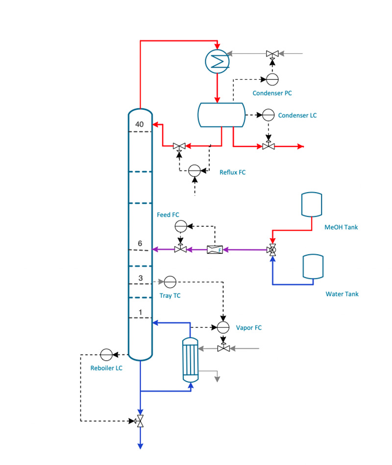
In my previous post I introduced the use of the build system Gradle and showed how it can be used to build Kotlin applications. As an example, I created a new project, “ColumnSimulation”, aimed at simulating a distillation column with a realistic control system. The column with its controls are shown in the picture below.

Binary distillation column separating methanol and water.

This is a conventional distillation column separating a 50/50 mixture of methanol and water. It has a total of 40 trays with 75% tray efficiency. Feed enters on tray 6 and the temperature on tray 3 is measured and controlled.

The system has 7 controllers where two are operated in a cascade arrangement (the Tray TC and the Vapor FC).

Object-Oriented Modeling

I use an object-oriented approach to modeling in order to retain maximum flexibility and code reusability. Thus, all units you see in the picture are represented by software classes stored in my SyMods library. In other words, the tray section, the reboiler, the condenser, the feed system, and the controllers are all units that can be configured for the application at hand. I’ve even combined the tray section, the reboiler and the condenser into a composite class called a “ColumnWtotalCondenser”. This saves me a bit of configuration effort every time I need a column of that type.

Given that I have all the pieces to the simulation pre-made, what remains to be done? I need to instantiate the classes into objects, configure them and make the connections corresponding to the process diagram. During this effort it is useful to do further grouping such as collecting all the controllers into another composite class called DCS (short for distributed control system). Notice that I use the Builder pattern to configure my controllers. There are other ways of doing this in Kotlin but the builder pattern is generic and works well in situations with many parameters. Also please note that the code type says “Swift” and not Kotlin. At this point Kotlin was not an option and Swift is sufficiently close in its syntax not to confuse the keywords of Kotlin too much.

class DCS: DCSUnit() {
    val feedFlowController = PIDController.Builder().
        gain(0.2).
        resetTime(0.002).
        directActing(false).
        pvMax(3000.0).
        sp(1634.0).
        output(0.25).
        build()
    val trayTemperatureController = PIDController.Builder().
        gain(0.75).
        resetTime(0.3).
        analyzerTime(0.025).
        pvMax(150.0).
        sp(92.0).
        directActing(false).
        output(0.5).
        build()
    val boilupFlowController = PIDController.Builder().
        gain(0.2).
        resetTime(0.01).
        analyzerTime(0.0).
        pvMax(2000.0).
        sp(1319.0).
        directActing(false).
        output(0.33).
        build()
    val reboilerLevelController = PIDController.Builder().
        resetTime(0.5).
        output(0.5).
        build()
    val condenserLevelController = PIDController.Builder().
        resetTime(0.5).
        pvMax(110.0).
        output(0.25).
        build()
    val condenserPressureController = PIDController.Builder().
        resetTime(0.1).
        output(0.5).
        pvMax(2.0).
        sp(1.0).
        build()
    val refluxFlowController = PIDController.Builder().
        gain(0.2).
        resetTime(0.002).
        analyzerTime(0.0).
        directActing(false).
        pvMax(3200.0).
        sp(831.0).
        output(0.25).
        build()
    init {
        with(controllers) {
            add(feedFlowController)
            add(trayTemperatureController)
            add(boilupFlowController)
            add(reboilerLevelController)
            add(condenserLevelController)
            add(condenserPressureController)
            add(refluxFlowController)
        }
    }
}

This took care of the control system setup. Next I configure the rest of the process by creating two reference fluid objects and instantiating the two process objects (Feeder and Column). The so-called reference fluids (refVapor and refLiq) are made in two steps. The first step is to instantiate a local dictionary object, factory, from a component file I’ve created using publicly available databases. In the second step I call a member function on the factory object with the names of the components I wish to include. The function searches a hard coded dictionary of Wilson activity parameters and creates an ideal vapor phase and a non-ideal liquid phase. These fluids are used as templates in all objects that require them. Finally, I connect the controllers to the process. All of that is part of the model class below.

class ProcessModel(var dcsUnit: DCS) {
    val ode = ODEManager()
    val factory = FluidFactoryFrom("/Users/bjorntyreus/component_file2.csv")
    val vl = factory.makeFluidsFromComponentList(listOf("Methanol", "Water"))
    val refVapor = vl?.vapor ?: throw IllegalStateException("Did not get a vapor")
    val refLiq = vl?.liquid ?: throw IllegalStateException("Did not get a liquid")

    val feed = Feeder(identifier = "Feed",
        composition = listOf(0.5, 0.5),
        initialFlow = 1600.0,
        minFlow = 0.0,
        maxFlow = 2000.0,
        operatingTemperature = 100.0,
        maxTemperature = 100.0,
        operatingPressure = 1.2,
        maxPressure = 3.0,
        refVapor = refVapor,
        refLiquid = refLiq)
    val column = ColumnWtotalCondenser(identifier = "column",
        numberOfTrays = numberOfTrays,
        feedRate = 1600.0,
        distillateRate = 800.0,
        refluxRatio = 1.0,
        topPressure = 1.0,
        trayDP = 0.005,
        trayEfficiency = 0.75,
        coolantInletTemperature = 25.0,
        trayDiameter = 3.0,
        lightKey = "Methanol",
        heavyKey = "Water",
        refVapor = refVapor,
        refLiq = refLiq)
    init {
        with(ode.units) {
            add(feed)
            add(column)
            add(dcsUnit)
        }
        column.trays[feedTrayLocation].liquidFeed = feed.liquidOutlet

        with(dcsUnit) {
            trayTemperatureController.pvSignal = column.trays[temperatureTrayLocation].temperatureTT
            trayTemperatureController.outSignal = boilupFlowController.exSpSignal
            trayTemperatureController.efSignal = boilupFlowController.normPvSignal
            boilupFlowController.slave = true

            boilupFlowController.pvSignal = column.reboiler.vaporBoilupFT
            boilupFlowController.outSignal = column.reboiler.heatInputAC
            boilupFlowController.efSignal = column.reboiler.heatInputAC
            column.reboiler.heatInputAC.useProcessInput = false

            reboilerLevelController.pvSignal = column.reboiler.levelLT
            reboilerLevelController.outSignal = column.reboiler.outletValveAC
            reboilerLevelController.efSignal = column.reboiler.outletValveAC
            column.reboiler.outletValveAC.useProcessInput = false

            feedFlowController.pvSignal = feed.feedRateFT
            feedFlowController.outSignal = feed.feedValveAC
            feedFlowController.efSignal = feed.feedValveAC
            feed.feedValveAC.useProcessInput = false

            condenserLevelController.pvSignal = column.condenser.levelLT
            condenserLevelController.outSignal = column.condenser.outletValveBAC
            condenserLevelController.efSignal = column.condenser.outletValveBAC
            column.condenser.outletValveBAC.useProcessInput = false

            condenserPressureController.pvSignal = column.condenser.pressurePT
            condenserPressureController.outSignal = column.condenser.coolantValveAC
            condenserPressureController.efSignal = column.condenser.coolantValveAC
            column.condenser.coolantValveAC.useProcessInput = false

            refluxFlowController.pvSignal = column.condenser.liquidOutletAFT
            refluxFlowController.outSignal = column.condenser.outletValveAAC
            refluxFlowController.efSignal = column.condenser.outletValveAAC
            column.condenser.outletValveAAC.useProcessInput = false
        }

    }
}

Notice how each controller connection requires four actions: 1) The controlled signal needs to be connected (pvSignal). 2) The output from the controller needs to be connected (outSignal). 3) The external feedback signal is then connected (efSignal). Often this signal is the same as the final control element except in cascade arrangements. 4) We have to make sure that the final control element responds to the attached control signal as opposed to retaining whatever process value that is given to it (e.g. during initialization).

We now have a process with its control system attached. Time to subject these to the integration system, prepare for data collection and design a test suite. This is done in the columnSimulation function below. Notice in particular how transparent it is to specify the timing for various tests by using Kotlin’s when expression in conjunction with ranges. It should be pretty clear from the code that during the span of 16 hours we are subjecting the process to the following changes:

  • Boilup controller switching from Auto to Cascade
  • Tray TC switching from Auto to Manual
  • ATV test on Tray TC
  • Tray TC back to Auto
  • Tray TC setpoint change 92 -> 85 oC
  • Applied results from ATV test and changed setpoint back to 92 oC
  • Feed composition change from 50/50 to 40/60 methanol/water
  • Feed flow increase by roughly 10%
fun columnSimulation(discr: DiscretizationModel, control: StepSizeControlModel): List<Plot> {
    // Prepare process for integration
    val dcsUnit = DCS()
    val model = ProcessModel(dcsUnit)
    val ode = model.ode
    
    // Instantiate, configure and start integrator
    val ig = IntegrationServer(discr, control)
    val dim = ode.dimension()
    val x = DoubleArray(dim)
    val endTime = 16.0
    ig.ode = ode
    ig.initialStepSize = 1.0e-3
    val reportingInterval = 0.05
    val dt = reportingInterval / 2.0
    var localTime = 0.0
    var reportTimer = 0.0
    ig.startTime = 0.0
    ig.start(ode.initialConditionsUsingArray(x))
    
    // Create lists to hold the dynamic data from a run
    val timeList = mutableListOf<Double>()
    val tempList = mutableListOf<Double>()
    val pressureList = mutableListOf<Double>()
    val tcOutList = mutableListOf<Double>()
    val boilupList = mutableListOf<Double>()
    val reboilLevelList = mutableListOf<Double>()
    val condenserLevelList = mutableListOf<Double>()
    val h20OHList = mutableListOf<Double>()
    val meohBtmsList = mutableListOf<Double>()
    val btmsFlowList = mutableListOf<Double>()
    val distList = mutableListOf<Double>()
    val feedRateList = mutableListOf<Double>()
    val feedCmpList = mutableListOf<Double>()
    val plotList = mutableListOf<Plot>()
    var atvGain = dcsUnit.trayTemperatureController.gainATV
    var atvReset = dcsUnit.trayTemperatureController.resetTimeATV
    var reductFactor = dcsUnit.trayTemperatureController.resetReductionFactor

    // Simulate and collect data
    while (localTime <= endTime) {
        localTime = ig.currentTime
        ig.startTime = localTime
        ig.endTime = localTime + dt
        ig.continueCalculations()
        localTime = ig.currentTime
        reportTimer += dt
        if (reportTimer > reportingInterval) {
            reportTimer = 0.0
            //println("time= $localTime, Tank temp = ${model.tank.tankTemperatureTT.processValue}")
            timeList.add(localTime)
            tempList.add(model.column.trays[temperatureTrayLocation].temperatureTT.processValue)
            pressureList.add(model.column.condenser.pressurePT.processValue)
            val tcOut = model.dcsUnit.trayTemperatureController.outSignal?.signalValue ?: 0.0
            tcOutList.add(tcOut * 100.0)
            boilupList.add(model.column.reboiler.vaporBoilupFT.processValue)
            reboilLevelList.add(model.column.reboiler.levelLT.processValue)
            condenserLevelList.add(model.column.condenser.levelLT.processValue)
            h20OHList.add(model.column.condenser.liquidHoldup.weightFractions[1] * 1.0e6)
            meohBtmsList.add(model.column.reboiler.reboilerHoldup.weightFractions[0] * 1.0e6)
            btmsFlowList.add(model.column.reboiler.outletFlowFT.processValue)
            distList.add(model.column.condenser.liquidOutletBFT.processValue)
            feedRateList.add(model.feed.feedRateFT.processValue)
            feedCmpList.add(model.feed.feedComposition[0] * 100.0)

            // Perform test on the system at specified time points
            val wholeHours = localTime.toInt()
            with (dcsUnit) {
                when (wholeHours) {
                    in 1..3 -> boilupFlowController.controllerMode = ControlMode.cascade
                    in 3..4 -> {
                        trayTemperatureController.controllerMode = ControlMode.manual
                        trayTemperatureController.output = 0.92
                    }
                    in 4..6 -> {
                        trayTemperatureController.h = 0.10
                        trayTemperatureController.controllerMode = ControlMode.autoTune
                        atvGain = trayTemperatureController.gainATV
                        atvReset = trayTemperatureController.resetTimeATV
                        reductFactor = trayTemperatureController.resetReductionFactor
                    }
                    in 6..7 -> {
                        trayTemperatureController.controllerMode = ControlMode.automatic
                        trayTemperatureController.sp = 92.0
                    }
                    in 7..8 -> {
                        trayTemperatureController.controllerMode = ControlMode.automatic
                        trayTemperatureController.sp = 85.0
                    }
                    in 8..9 -> {
                        trayTemperatureController.gain = atvGain / 2.0
                        trayTemperatureController.resetTime = atvReset
                        trayTemperatureController.sp = 92.0
                    }
                    in 10..12 -> {
                        model.feed.currentComposition = listOf(0.4, 0.6)
                    }
                    in 12..14 -> feedFlowController.sp = 1800.0
                }
            }
        }
    }

The actual start of the program is trivially simple. In the main function I call the columnSimulation function and get a list of plots back. Six of these I display in one figure and the other six go to the second figure. The whole operation of simulating the 40 tray column for 16 hours takes 1.6 seconds on a 2014 vintage MacBook Pro. Kotlin is fast!

fun main(args: Array<String>) {
    val timeInMillis = measureTimeMillis {

        val plotGroup = columnSimulation(DiscretizationModel.ModifiedEuler, StepSizeControlModel.FixedStepController)

        val group1 = plotGroup.take(6)
        val group2 = plotGroup.drop(6)
        gggrid(group1, ncol = 2, cellWidth = 470, cellHeight = 300).show()
        gggrid(group2, ncol = 2, cellWidth = 470, cellHeight = 300).show()

    }
    println("(The operation took $timeInMillis ms)")
}

Below I show the results of the simulation run described in the code.

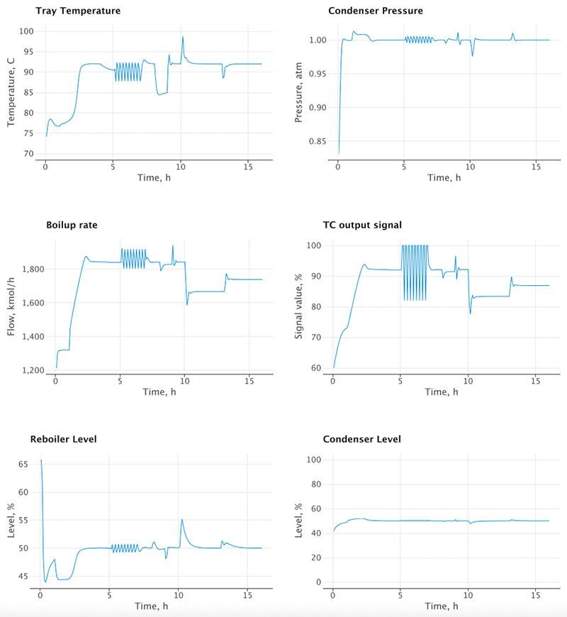
Performance of control system for the 40 tray column. Pay particular attention to the Tray Temperature Controller behavior (upper left). It is activated (cascade with Boilup) after 1 hour of operation but responds slowly due to poor tuning. After the ATV test the old tuning parameters remain for one setpoint change (at hour 7). The new tuning parameters are set at hour 8 just before a final setpoint change to 92 oC. After that both feed composition and feed rate change in steps of 10%. Temperature is held close to setpoint in the face of these disturbances.
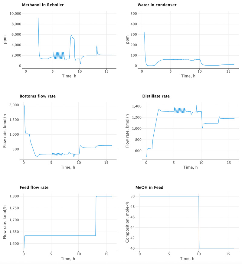
This figure shows how the important composition variables behave in the face of temperature setpoint changes and external disturbances. Notice that the ATV test itself causes only minor deviations in the compositions. The control system is also quite robust against feed rate and composition changes.

MVC

An important concept in software engineering is the separation of a Model from its View and the software Controller used to manipulate both the view and the model. The Model-View-Controller (MVC) concept is important because it enables software reuse, provides flexibility in the choice of views and controllers and it facilitates trouble shooting and debugging.

While this post is primarily aimed at demonstrating modeling with Kotlin and Let’s plot, it also provides me with an opportunity to dwell a bit on MVC.

In the example above it should be clear that the model in my MVC is the class “ProcessModel”. It consists of the column, the feeder and the feedback control system. But the model does nothing by itself, it needs to be driven by an integrator and be told about changes to its environment. That’s the job of the controller.

Furthermore, the model has no built-in display capabilities or views. The reason is that you should be able to choose the view independently from the model. Only the controller will know about the view and will be feeding it with information from the model.

In my example the function columnSimulation(…) is the controller. It owns the model and the integrator and knows how to collect information to feed the plotting program Let’s plot. But we could have chosen another method to display the result. For example, the controller could have exported data to a text file that could have been used to display graphs in Excel. I have used that method many times.

To further drive home the flexibility of a well designed MVC I share an example simulation of the same distillation column on an iPad. Here the model is the same as above but implemented in Swift instead of Kotlin. However, the views and controllers are quite different. Instead of collecting data for static plots I update strip charts live as the simulation progresses. I also provide views and dedicated controllers for the PID controllers so the user can interact with them and provide tuning parameters while the simulation is running. This mode of operation is called interactive dynamic simulation and mimics running a real plant.

I’m currently exploring a user interface system (controllers and views) called TornadoFX. It has a set of Kotlin API’s for user interfaces and is built upon a well established UI system called JavaFX. I’m hoping to report progress on my findings in a future post.

Categories
Dynamic Modeling iOS MacOS Windows

Swift vs Python for Dynamic Simulation

Swift and Python are two programming languages I’ve recently used to write process models for interactive, dynamic simulations. They are both modern and powerful with Swift being the youngest; still evolving and improving. Python is very popular overall and has found use in a number of areas, more recently Machine Learning.

Both Python and Swift support Object-Oriented programming, which is essential for building modular dynamic simulation models. While the syntax for the two languages is different, it is still relatively straightforward to construct a function or a class in one language given the design in the other. But I must say that working from models implemented in Swift towards designs in Python seems easier than the other way around. This could have to do with the fact that Swift is strongly typed and Python is not.

The dynamic nature of Python makes it ideal for rapid construction and experimentation. You can create a class in Python, add some attributes and member functions (also called methods) and test it right away. This is because Python is an interpreted language. What that means is that the keywords and instructions you enter as your program are interpreted by the Python executable and then sent to various pre-compiled functions within the application for execution. The big advantage of this approach is that you don’t have to specify variable types (e.g. int, double, etc) you use; the interpreter figures that out for you from the context of how they are used. However, this flexibility comes at a cost. First, since variables are not explicitly typed there is little to no help or warnings given to you before you run the program. Although debugging is relatively easy, I often find that many errors made by me could readily have been caught by a compiler before I even attempted to hit the “run” button.

The second, and possibly most serious drawback of an interpreted language is execution speed. This is particularly true for simulations of complex models with plenty of math. While there are some areas of computation where execution speed is of secondary importance compared to flexibility, the area of dynamic simulations is not one of them.

At this point you might wonder why I even considered Python for dynamic simulations instead of using fast languages like C++, C#, and Java. And certainly, 20-30 years ago those were my work horses. But back then computers were a lot slower than they are today and every bit of help from a compiled language was needed in order to make an interactive simulation fast enough to be useful. Today the situation is different. Most laptops or even tablets are fast enough to run an interactive, dynamic simulation written in Swift or Python at an acceptable speed. Notice the emphasis on interactive. It means that a process simulation runs much faster than real time but not so fast that you the “operator” don’t have time to interact to make changes. Here is an example of what I’m talking about.

Example of an interactive, dynamic simulation running on an iPad and written in Swift.

So with today’s computers Python cannot be dismissed solely on the basis of execution speed. And once we decide to keep it in the running we can focus on the many advantages offered by the language itself and its rich set of libraries. One of those is the plotting library Matplotlib (https://matplotlib.org). The library is described on its website in one sentence: “Matplotlib is a comprehensive library for creating static, animated, and interactive visualizations in Python”. I would add that it is powerful and easy to use. And very importantly, like Python itself, it’s open source and freely available. You will find many examples in my blogs of how I use Matplotlib in my own research.

In addition to Matplotlib the other library that is practically mandatory for dynamic simulations is NumPy (https://numpy.org). The single sentence characterization of this library is: “The fundamental package for scientific computing with Python”. NumPy is a set of routines written in C that significantly boosts the speed of mathematical expressions used to write dynamic simulation models. In my code examples you will see how I practically always use NumPy.

Another area of great importance for interactive, dynamic simulations is graphical user interfaces (GUI). If you are writing code in Swift for iOS devices you get help in creating slick interfaces from the tools in Apple’s development environment, Xcode. Personally I have never found it particularly easy to get it exactly right but it’s probably my old desktop/laptop background getting in the way of modern iOS thinking. Presumably for the same reasons I have found it easier to work with some of the external libraries that integrate with Python, for example PyQt5 (https://pypi.org/project/PyQt5/ ). This library contains a set of graphical interface routines written in C++ with a Python API. I will show in a separate blog how I have used PyQt5 to build a flexible and reusable interface for dynamic simulations.

It may feel that I’m writing mostly about Python, almost to justify its use. This is partly true because Swift does not need much in terms of justification, Apple got it right from the beginning. Swift not only supports Object-oriented programming but also advocates what they call protocol oriented designs. A Swift protocol is like a C++ or Java interface (if that helps anybody?) and does not have a direct counterpart in Python. Python’s abstract base class has some features along the lines of an interface, but not really. And Swift’s protocols are quite powerful, even more so than a classic Java interface. In fact, you can create a whole design based just on protocols that can later be implemented in various ways.

Swift is a strongly typed and compiled language. What that means is that all class variables you introduce must be of some type (e.g. Int, Double, some class or even a protocol) and be initialized before they are cleared for compilation. This is a huge advantage since you are guaranteed not to send messages to objects that can’t receive them. Of course you can still make logical mistakes just like you can in all programming languages. But that’s up to you and a good debugger to figure out. The compilation into machine code, and linking with runtime libraries, is not overly fast but once your program is compiled it is really fast! We are talking about orders of magnitude faster than Python especially for simulation tasks. And that is with use of NumPy. Surely you can take steps to speed up your Python code but now you have lost some time in development, made the code a little more fragile and perhaps lost some generality. Swift is consistently fast right from the get go.

Now you might think that Swift is the clear winner? Well, if runtime speed were everything it would be. But there are other considerations. While Swift has been made open source (https://www.swift.org) it is still very young and does not yet have nearly the same eco system of support that Python has. What I’m especially missing today is a good plotting package, like Matplotlib, that is freely available and integrates readily with Swift on all platforms. It will come, I’m sure.

Swift was designed by Apple to replace Obj-C, their other language for which many excellent libraries were written. When you run Swift on iOS and OS X devices you take advantage of all that code and enjoy great performance. The open source team is porting Swift (both development and runtime) to other platforms like Windows. I have not tried Swift on Windows yet but I know that Python runs equally well on both platforms.

Conclusions

Swift and Python are both excellent programming languages for writing dynamic simulation models. Both being modern emphasize “people time” over run time. Python is senior to Swift and enjoys a rich set of high quality, open source libraries. Swift is strongly typed, logical and fast. I use both in my work and research. For production and customer requested models I prefer Swift. For my own research and experimentation I prefer Python. Most of my process models are implemented in both languages, developed and tested in one language first and then ported to the other.